Vertex Connection and Merging

I implemented vertex connection and merging (VCM) in my renderer. VCM is an extension of bidirectional path tracing (BPT) that adds a family of biased sampling techniques. These sampling techniques form full paths by effectively fusing a light subpath vertex with an eye subpath vertex, rather than connecting the two vertices with an edge. These new merging sampling techniques are formulated in the path integral framework so that they can be combined with the existing connection sampling techniques of BPT and with each other using multiple importance sampling (MIS).

The measurement contribution function of paths created using merging is straightforward to compute. It approximates the unbiased measurement contribution function described by Veach, except that at the merging location, it uses the BSDF of the last eye subpath vertex evaluated with incoming direction determined by the last edge of the light subpath (alternatively, the direction from the last eye subpath vertex to the second last light subpath vertex could be used). The probability density of sampling the path is the probability density of the connection technique with one fewer light subpath vertices times an acceptance probability: the probability with respect to area of sampling a point on a disk with a specified radius centered at the last eye subpath vertex. This acceptance probability is computed by integrating the probability density with respect to area (or with respect to projected solid angle, as in my implementation) over that disk. For a relatively small disk, this integral can be approximated by taking the probability density with respect to area of one point in the disk multiplied by the area of the disk.

Assuming that large numbers of vertices are made available for merging, the resulting algorithm combines the strengths of BPT and photon mapping, automatically weighting the contributions of the various sampling techniques to produce the minimum amount of noise. In particular, VCM allows specular–diffuse–specular (SDS) paths to be discovered efficiently.

I also implemented a technique that allows the MIS weights to be computed efficiently using only data stored at the two vertices being connected or merged. This technique is not particularly intuitive but it can be derived mathematically. I made just a few modifications including adding support for direct sensor hits.

Below are some renders of a blue plastic ball embedded in a clear plastic ball, lit by a small bright light. Click the images to view them at full size.

BPT

VCM (equal time)

VCM, weighted merging contribution

VCM, weighted connection contribution (including direct light and sensor hits)

VCM, weighted contribution of unidirectional path tracing with direct light sampling

Below are some renders of a room lit by a lamp bounced off a mirror ceiling.

BPT

VCM (equal time)

VCM, weighted merging contribution

VCM, weighted connection contribution (including direct light and sensor hits)

VCM, weighted contribution of unidirectional path tracing with direct light sampling

Bidirectional Path Tracing Enhancements

Several months ago, I implemented a couple additional bidirectional path tracing features described in Veach's thesis. Specifically, I added support for ideal specular BSDFs and support for special direct illumination sampling strategies. Below are some renders illustrating these features. Click the images to view them at full size.

Specular BSDFs:

The metallic ball, the smooth parts of the checkered glass ball, and the small glass ball use ideal specular BSDFs.

Direct illumination: 

Render without a special direct illumination sampling strategy.

Render with a special direct illumination sampling strategy. Samples are distributed uniformly over the solid angle subtended by the lights.

Indirect Light

Bidirectional path tracing is very good at rendering scenes lit primarily by indirect light. Unlike unidirectional path tracing, bidirectional path tracing can sample indirect light directly by connecting eye subpath vertices to any light subpath vertex, not just points on the light source itself. This allows the light source to be found even when it is not directly visible. Below is an image that illustrates this, rendered in my renderer using bidirectional path tracing.

Image rendered using bidirectional path tracing. Click image to view full size.

Below is the same render showing only the contribution of paths composed of two or more eye subpath vertices and zero or one light subpath vertices—the path types generated by a typical unidirectional path tracer with direct light sampling. Unidirectional path tracing can sample the light source efficiently only when it is directly visible. In the indirectly lit parts of the scene, especially those far from or multiple bounces away from the ceiling, it contributes very little compared to other sampling techniques. It isn't even the best sampling technique in the area of the ceiling closest to the light bulb, which is sampled most efficiently by light tracing.

Image rendered using bidirectional path tracing, but showing only the contribution of the
sampling techniques used by unidirectional path tracing with direct light sampling.

I modeled this scene in Maya, inspired by the indoor scene Veach used in his thesis.

SDS Paths

Although bidirectional path tracing can efficiently render many types of paths, it has a very difficult time rendering specular–diffuse–specular (SDS) effects (such as reflected and refracted caustics) because they can only be sampled with pure light tracing (t = 0) or pure eye tracing (s = 0). Metropolis light transport can render these types of paths much more efficiently because once it discovers one it can use small path mutations to explore similar paths, all in an unbiased way.

While testing these SDS paths in my renderer, I discovered a few other interesting things. First, when using certain algorithms, infinitesimal changes in primary sample space can result in large jumps in path space. These jumps can cause interesting but undesirable artifacts in parts of MLT renders where small-step mutations are key (such as the lighting of the blue sphere in the images below). Second, because bidirectional path tracing is so bad at rendering SDS images, even tens of millions of bidirectional path tracing samples are not enough to to compute an accurate estimate of the average scalar contribution. This can result in MLT renders that are slightly too bright or slightly too dark.

Below are some equal-time renders of a blue sphere inside an acrylic sphere. The first image was rendered using MLT, the second was rendered using MLT with an alternate method of computing an arbitrary orthonormal basis given a surface normal, and the third image was rendered using standard bidirectional path tracing. Both MLT and BPT make easy work of the caustic, but BPT has a hard time rendering the blue sphere, the caustic reflected from the lower left of the acrylic sphere, and other effects. Click the images to compare them at full resolution.

MLT

MLT with obvious mutation discontinuities

BPT

Below are some less converged versions of the images above: 

MLT

MLT with obvious mutation discontinuities

BPT

Improved MLT

I recently revisited my bidirectional path tracer and found a small bug in my Metropolis implementation. For choosing the location on the image plane I was accidentally using new random numbers instead of the special random numbers from my random number stream. This meant that the eye subpaths were not properly correlated, which was causing a major reduction in image quality. After fixing this bug, the benefits of MLT became much more apparent.

Below are some approximately equal-time renders for comparison, as well as a more converged reference image. The area most improved by the bug fix is probably the reflection on the glass ball. MLT now outperforms bidirectional path tracing everywhere except the dark areas of the image. You can use the lightbox to switch between images.

MLT after bug fix.

MLT before bug fix.

Bidirectional path tracing.

Pure unidirectional path tracing from the camera (s = 0, t ≥ 2).

High quality bidirectional path tracing reference.

Working Metropolis Light Transport

I just finished implementing Metropolis light transport (MLT) in my bidirectional path tracer. I will post more details later, but for now here's a very rough, quick summary and a few early test renders.

Rather than implementing Veach's path space MLT as I had originally planned, I decided to implement primary sample space MLT based on the paper by Kelemen et al. This algorithm works by mutating points in the "primary sample space", the space of random numbers that drive a Monte Carlo renderer.  Each point in this space maps to a particular path, and mutations in this space correspond to mutations in path space. The algorithm is very general because it works by manipulating the random number stream that drives the renderer rather than manipulating the paths themselves. Mutating paths directly can be relatively tricky.

A lot went into implementing MLT. I wrote a nice random number stream system, with lazy evaluation of random numbers and mutations. I made some significant modifications to my bidirectional path tracing core so that MLT could be added in an elegant way. I made a method to compute an approximate average scalar contribution for the entire image using a Halton sequence to distribute samples over the image (I use this when normalizing the results of the Metropolis sampling algorithm). And of course I implemented the Metropolis–Hastings algorithm.

In my renderer, bidirectional path tracing can now be run with or without MLT. Furthermore, I can continue adding features to the underlying bidirectional path tracer and they will automatically work with MLT enabled.

There are a number of optimizations that I plan to add to improve the rate of convergence, but for now I'm satisfied that the algorithm is working correctly and converges to the same results as regular bidirectional path tracing. MLT currently converges more slowly than bidirectional path tracing alone in most cases, but this should be fixed with a little more work. I also want to do some more testing.

Here are some early test renders. Click the images to view them at full size.

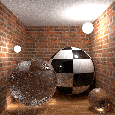
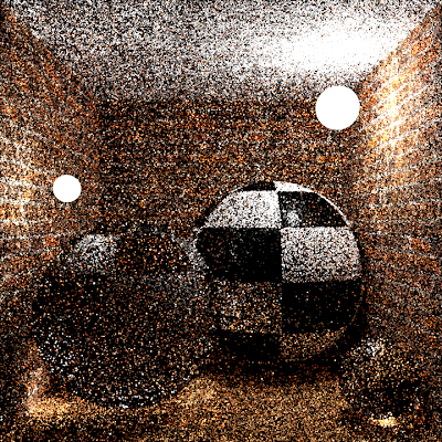
Kelemen MLT on top of bidirectional path tracing.

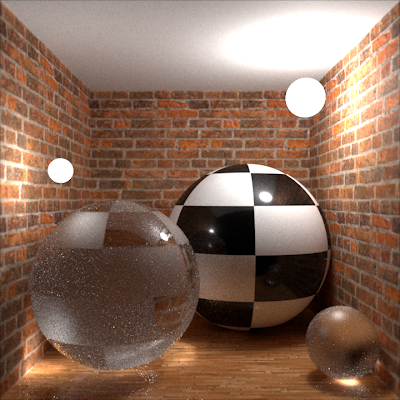
Bidirectional path tracing without MLT. Same number of samples as the image above.

A longer MLT render.

High quality bidirectional path tracing reference.

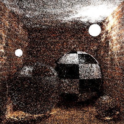
An MLT render with only local (small step) mutations. This image shows the expected streaky and clumpy artifacts that result from locally exploring the space.

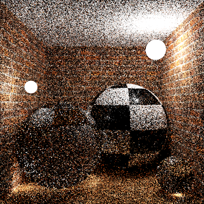
An MLT render with only global (large step) mutations. Same number of samples as the previous image.

An MLT render with both types of mutations. Same number of samples as the previous image.

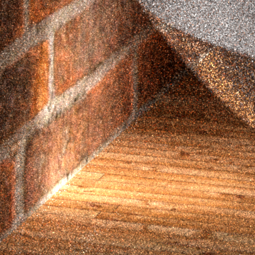
A close-up of a caustic rendered using MLT. While many parts of the image are noisier than the bidirectional path tracing version below, the bright caustic on the floor and wall are more converged.

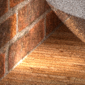
A close-up of a caustic rendered using bidirectional path tracing, with the same number of samples as the image above.

Complete MIS and Optimizations

I finished my multiple importance sampling (MIS) implementation by adding the one missing piece: correct evaluation of the probability density with respect to solid angle of sampling a particular direction from the sensor. I also added a few other important optimizations: Russian roulette for subpath termination, Russian roulette for connecting edge visibility tests, and light emission samples chosen according to the distribution of power over multiple lights. I tested everything very carefully along the way. An important variance reduction technique that I haven't yet implemented is support for special direct illumination strategies.

Below are two images that used the same number of samples and took the same amount of time to render. The difference is that one was rendered with MIS and the other was not (it was rendered by simply weighting the contribution of each path by one over the number of possible sampling techniques for a path of that length). These images illustrate how important MIS is for bidirectional path tracing. The remaining fireflies and severe noise in the MIS image are a result of rare SDS paths that bidirectional path tracing has trouble with. I will soon be implementing MLT in this renderer to help render these types of paths.

Bidirectional path tracing with MIS.

Bidirectional path tracing without MIS.

Microfacet BSDF for Reflection and Refraction

Last year I implemented (see my blog posts here and here) a microfacet model for reflection and refraction based on the 2007 paper by Walter, Marschner, Li, and Torrance. In order to port my implementation of this BSDF to my bidirectional path tracer, I needed to add a few features and make a few fixes. In particular, I needed to scale the radiance of light that is transmitted across the interface, I needed to prevent bad reflection and refraction directions, and I needed to add the ability to evaluate the probability density of sampling a given direction. I also had to track down and fix a couple minor bugs. After making these additions and fixes, the BSDF works great.

The following images compare the results of the microfacet BSDF and a simple ideal specular BSDF. They match very closely, as they should.

Glass balls using the microfacet BSDF with very low roughness, rendered in my bidirectional path tracer.

Glass balls rendered using ideal specular reflection and refraction, rendered in Photorealizer.

Of course, the cool thing about the microfacet BSDF is that it can be used for rough surfaces, not just smooth ones. For the following image I used the microfacet BSDF for both of the glass spheres. I modulated the roughness of the left sphere (between smooth glass and ground glass) using a procedural texture map. The roughness of the right sphere is in between the two roughness values used on the left sphere.

The glass spheres use the microfacet BSDF for reflection and refraction.

Here's another image that uses this BSDF with a fairly low roughness:

The glass monkey on the right uses the microfacet BSDF for reflection and refraction.

A close-up of the rough glass monkey.

Notice that, while these images are quite smooth overall, there is still some noise in the glass objects. This is because bidirectional path tracing cannot efficiently handle tricky SDS (specular–diffuse–specular) paths (in other words, reflected and refracted caustics). I am planning on implementing MLT soon, which will allow me to better handle these types of paths.

Disney Principled BSDF

I implemented the diffuse and specular parts of the Disney "principled" BRDF (slides, notes), a new multipurpose analytic BRDF from Walt Disney Animation Studios, created for Wreck-It Ralph and designed to match MERL measured data. The results look great. Below are a few images that I've rendered in my bidirectional path tracer using this BRDF.

For the following image I used the Disney "principled" BRDF for all of the surfaces except the two glass balls (and the lights and sensor).

An image I rendered in my bidirectional path tracer. All of the surfaces except the glass balls use the Disney "principled" BRDF.

For the following image, I used the Disney "principled" BRDF for the two monkeys in the middle, the wood and green plastic ones.

An image I rendered in my bidirectional path tracer. The wood and green plastic monkeys use the Disney "principled" BRDF.

A close-up of the wood and green plastic monkeys.

As usual, I haven't post-processed these images in any way outside my renderer, and you can click them to view them at full size.

Diffuse Reflection and Transmission BSDF

My improved BSDF system is very general and makes it really easy to add new BSDFs that contain any kind of reflection and transmission. To test this, I implemented a constant BSDF of 1/(2π). It's defined over the entire sphere, so it diffusely reflects half of the incident light and diffusely transmits the other half.

I rendered the image below in my bidirectional path tracer. The blue monkey on the left uses this new constant BSDF, giving it a soft and translucent appearance (putting a light behind the monkey would illustrate the translucency better). My next couple blog posts will describe the BSDFs I used for the other monkeys in this image.

The blue monkey on the left uses this constant-valued, reflecting and transmitting BSDF.

A close-up of the blue monkey.

Multiple Light Sources

I added support for multiple light sources to my bidirectional path tracer. For now, when selecting an origin light for the light subpath, all of the lights are chosen with equal probability, but I will soon make the probability of selecting a particular light proportional to its total emitted power.

One light source.

Two light sources, same total power.

Two different colored light sources, same total power.